Why I Joined Wherobots Plus A Look At Apache Sedona
William Lyon
October 18, 2023
20 min read
I recently joined a new company, Wherobots, where I will be leading Developer Relations efforts to help developers and data scientists work with spatial data. In this post I wanted to share a bit about why I'm so excited about not just Wherobots but the spatial data analytics space in general, plus we'll take a brief look at Apache Sedona, the technology at the foundation of the cloud-native geospatial analytics database that Wherobots is building.
Stay Updated
Get notified about new posts and videos
Starting A New Adventure At Wherobots#
I shared a bit on LinkedIn about why I decided to join Wherobots (as one does), but I wanted to go into a bit more details here. Wherobots was founded by the creators of the Apache Sedona open-source project, which brings geospatial functionality to distributed computing frameworks like Apache Spark and Apache Flink. Wherobots is building a cloud-native geospatial analytics and AI database engine using Apache Sedona as a foundational piece of that architecture.
The key sentence in my LinkedIn post above that addresses the "Why Wherobots?" question is this:
Fundamentally I believe that the world's most pressing problems are geospatial in nature and Wherobots is at the center of emerging trends in geospatial data analytics.
Let me elaborate on that with a bit of a personal journey. I live in the North West of the United States. The summer of 2020 was particularly bad for wildfires in the area and at the end of August, after hiding indoors for most of the summer my wife and I looked at a smoke forecast map to find somewhere we could escape to for a few weeks to avoid the smoke and reclaim a bit of our summer. We found a fun little AirBnb in the woods away from wildfire smoke and had a nice time breathing fresh air for a bit.
On the bookshelf of our little rental cabin was a Charles Mann book "The Wizard and the Prophet" which I started reading. I won't summarize the entire book here but it deals with conflicting approaches of how technology can play a role in helping humanity thrive. Reading this book in the rainforest next to a national park where I had escaped smoke from wildfires, this book had a profound impact on me as it became so apparent that spatial data was at the heart of many of the most important challenges for humanity.
But spatial data is also at the heart of so many day to day decisions and applications we interact with regularly. Consider my challenge of finding an affordable rental cabin with WiFi in an area where the risk of wildfire smoke was low for a period of time. Or figuring out where you can go hiking with minimal wildfire risk (I call this category of problem "Adventure Planning In The Anthropocene") Spatial data problems are literally everywhere.
I've always been interested in geospatial data tooling. Some of the first work I did with Neo4j was a Google Summer of Code project adding spatial support to Cypher (Neo4j's query language) and since then I've tried to share what I've learned in the world of working with geospatial data such as creating heatmaps of offshore company owners, spatially analyzing US Congress, implementing spatial search functionality, working with geospatial data in Neo4j, building routing web apps with OpenStreetMap data, making sense of geospatial data with knowledge graphs, building geospatial GraphQL APIs, applying graph algorithms to analyze the physical world, or working with the new Overture Maps dataset.
When I first started talking with the Wherobots co-founders, Mo and Jia, and they shared their vision with me of building a cloud-native spatial analytics and AI database I knew I wanted to be a part of it. Wherobots is exciting to me not just because of the amazing technical challenges of building a cloud-native data platform but Wherobots is also at the center of emerging trends in technology at large. There are currently monumental shifts in the earth observation industry enabling entirely new use cases, cloud-native analytics is synthesizing into a composable data stack, and a recent inflection point in AI and machine learning is forcing a re-think of how we work with data at every layer of the stack. Wherobots is at the intersection of these important trends.
Spatial data problems are all around us and I'm excited to be working at the intersection of these exciting trends.
Apache Sedona Docker Quickstart#
Wherobots was founded by the creators and core contributors to the Apache Sedona open-source project so I thought it was important to become as familiar with Apache Sedona as I could. I'm a firm believer that the best way to learn something completely is to help others understand it so I recorded a short video introducing Apache Sedona and showing how to get started with Apache Sedona using Docker.
What Is Apache Sedona?#
Apache Sedona is an open-source framework for working with large scale geospatial data. It adds spatial functionality to distributed data processing frameworks like Apache Spark and Apache Flink to enable developers and data scientists to work with spatial data at scale.
Apache Sedona exposes native types for representing complex geometries like points, lines, and polygons and implements geospatial indexing and partitioning for fast lookups and efficient distributed processing of spatial data at scale. Geospatial querying functionality is available with SQL (SedonaSQL) by implementing the SQL-MM3 and OGC SQL standards.
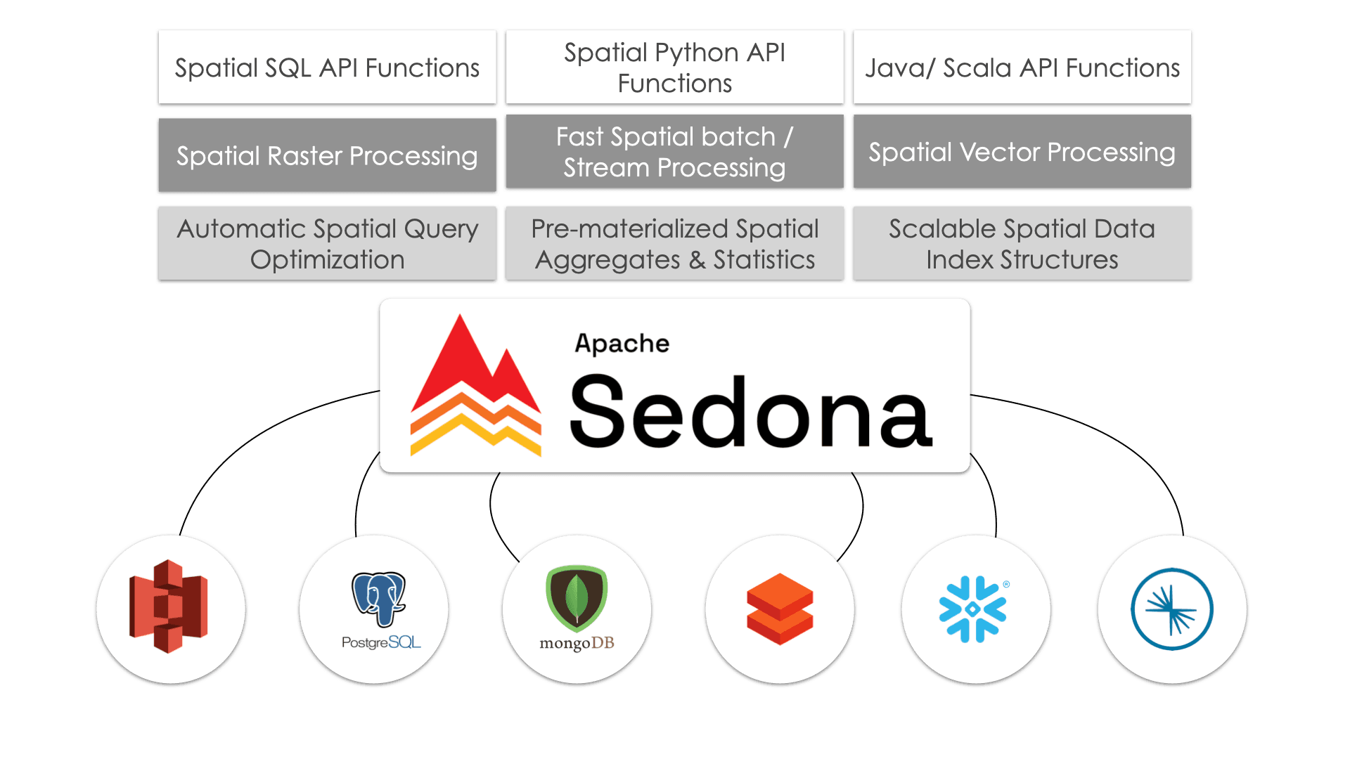
We can work with Apache Sedona via Python, R, SQL, and other tooling - such as a Jupyter Notebook environments and via seamless integration with the PyData ecosystem.
There are many ways to leverage Apache Sedona whether incorporating into an existing data pipeline or building a new greenfield analytics application. For example Apache Sedona can be deployed into a Databricks cluster, run in AWS EMR, it works with Snowflake, or can be run on your own infrastructure. In this post we'll be using the Apache Sedona Docker image to get a cluster running locally and perform some basic geoprocessing tasks.
Apache Sedona Docker Image#
First, we'll pull down the latest version Docker image:
docker pull apache/sedona:latest
Then let's run a new container from this image:
docker run -p 8888:8888 -p 8080:8080 -p 8081:8081 -p 4040:4040 \
-v $(pwd)/geodata:/opt/workspace/geodata \
apache/sedona:latest
A few things to note about this command:
- We're exposing a few ports from the container to our local machine, notably
8888for the Jupyter environment,8080for the Spark cluster web UI,8081for the Spark worker UI and4040for the Spark job UI - We're mounting a volume in the container to map to
~/geodataon my local machine. I have some Shapefiles stored in this directory and I'd like to access them via Sedona, execute some geoprocessing steps, and then write back to that directory.
This docker command will start a local Apache Spark cluster in the container with Apache Sedona installed, as well as a Jupyter environment that we'll use as the primary interface for working with Apache Sedona. If we open localhost:8888 in a web browser we'll see a JupyterLab environment. The Apache Sedona docker image includes a few existing notebooks to demonstrate some of the features of Apache Sedona. Let's first take a look at these existing notebooks and then we'll create a new notebook to run our geoprocessing tasks.
ApacheSedonaCore.ipynb#
The first notebook we'll look at is ApacheSedonaCore.ipynb which demonstrates how to interact with Apache Sedona using the core RDD API. Apache Sedona introduces new objects that extend the concept of Spark's Resilient Distributed Dataset (RDD) with "Spatial RDDs" which are essentially spatially aware RDDs. Spatial RDDs have a specific geometry type associated with them (Point, Line, Polygon, Circle, Rectangle etc) and expose spatially specific operations.
Creating A Spatial RDD
For example, here we create two spatial RDDs from csv files, specifying RectangleRDD and PointRDD respectively.
rectangle_rdd = RectangleRDD(sc, "data/zcta510-small.csv", FileDataSplitter.CSV, True, 11)
point_rdd = PointRDD(sc, "data/arealm-small.csv", 1, FileDataSplitter.CSV, False, 11)
Spatial Indexes & Partitions
One key feature of Apache Sedona is introducing spatial partitioning which efficiently controls how data is distributed across the cluster. Spatial indexes ensure fast lookups and efficient spatial operations.
Here we specify spatial partitions and build a spatial index for our spatial RDDs. For spatial partitioning we can choose from KDB-Tree, Quad-Tree, and R-Tree and for spatial indexes we can choose between Quad-Tree and R-Tree.
point_rdd.spatialPartitioning(GridType.KDBTREE)
point_rdd.buildIndex(IndexType.RTREE, True)

rectangle_rdd.spatialPartitioning(point_rdd.getPartitioner())
Spatial Operations
Next, let's see some of the types of spatial operations available with the core RDD API. Later we'll see how to leverage SQL for similar functionality.
Spatial Join
Here we perform a spatial join, joining our point spatial RDD with the rectangle spatial RDD, then create a DataFrame from the result set.
result = JoinQuery.SpatialJoinQueryFlat(point_rdd, rectangle_rdd, False, True)

spatial_join_result = result.map(lambda x: [x[0].geom, x[1].geom])
sedona.createDataFrame(spatial_join_result, schema, verifySchema=False).show(5, True)
+--------------------+--------------------+
| geom_left          |          geom_right|
+--------------------+--------------------+
|POLYGON ((-87.229...|POINT (-87.204299...|
|POLYGON ((-87.082...|POINT (-87.059583...|
|POLYGON ((-87.082...|POINT (-87.075409...|
|POLYGON ((-87.082...|POINT (-87.08084 ...|
|POLYGON ((-87.092...|POINT (-87.08084 ...|
+--------------------+--------------------+
only showing top 5 rows
Spatial KNN Query
A spatial KNN query is an operation that searches for the k nearest neighbors. Here we can search for the 5 points in our point spatial RDD nearest to an arbitrary point.
result = KNNQuery.SpatialKnnQuery(point_rdd, Point(-84.01, 34.01), 5, False)
Spatial Range Query
Spatial range queries typically involve finding all geometries in a dataset (in this case a spatial RDD) that intersect with a given range, or query window. Here we search for all geometries from our line spatial RDD that intersect with a given boundary.
query_envelope = Envelope(-85.01, -60.01, 34.01, 50.01)

result_range_query = RangeQuery.SpatialRangeQuery(linestring_rdd, query_envelope, False, False)
Next, let's explore using Sedona via SQL. We'll take a look at the ApacheSedonaSQL_SpatialJoin_AirportsPerCountry.ipynb notebook.
ApacheSedonaSQL_SpatialJoin_AirportsPerCountry.ipynb#
In addition to the core API, Apache Sedona also supports SQL. Specifically, a flavor of SQL that adds functions for spatial operations consistent with the MM3 and OGC Spatial SQL specifications called SedonaSQL. These are typically additional functions in SQL prepended with ST_ (here ST stands for spatio-temporal) which are typically used for vector operators and RS_ for working with raster data.
In this notebook we import data containing country boundaries and airport locations. Then we'll join them together using a spatial join operation and use a GROUP BY operation to compute the number of airports in each country - all using SQL!
First we import our data on countries and airport, in this case from two shapefiles.
countries = ShapefileReader.readToGeometryRDD(sc, "data/ne_50m_admin_0_countries_lakes/")
countries_df = Adapter.toDf(countries, sedona)
countries_df.createOrReplaceTempView("country")


airports = ShapefileReader.readToGeometryRDD(sc, "data/ne_50m_airports/")
airports_df = Adapter.toDf(airports, sedona)
airports_df.createOrReplaceTempView("airport")
We saw an example above of a spatial join operation using the core RDD API, let's now see how we can run a spatial join using SedonaSQL. We'll combine countries and airports where the airport point geometry is contained within the boundaries of a country's polygon geometry using the ST_Contains SQL predicate.
result = sedona.sql("SELECT c.geometry as country_geom, c.NAME_EN, a.geometry as airport_geom, a.name FROM country c, airport a WHERE ST_Contains(c.geometry, a.geometry)")
+--------------------+--------------------+--------------------+--------------------+
| country_geom       | NAME_EN            | airport_geom       |                name|
+--------------------+--------------------+--------------------+--------------------+
|MULTIPOLYGON (((1...|Taiwan ...          |POINT (121.231370...|Taoyuan ...         |
|MULTIPOLYGON (((5...|Netherlands ...     |POINT (4.76437693...|Schiphol ...        |
|POLYGON ((103.969...|Singapore ...       |POINT (103.986413...|Singapore Changi ...|
|MULTIPOLYGON (((-...|United Kingdom ...  |POINT (-0.4531566...|London Heathrow ... |
|MULTIPOLYGON (((-...|United States of ...|POINT (-149.98172...|Anchorage Int'l ... |
|MULTIPOLYGON (((-...|United States of ...|POINT (-84.425397...|Hartsfield-Jackso...|
|MULTIPOLYGON (((1...|People's Republic...|POINT (116.588174...|Beijing Capital ... |
|MULTIPOLYGON (((-...|Colombia ...        |POINT (-74.143371...|Eldorado Int'l ...  |
|MULTIPOLYGON (((6...|India ...           |POINT (72.8745639...|Chhatrapati Shiva...|
|MULTIPOLYGON (((-...|United States of ...|POINT (-71.016406...|Gen E L Logan Int...|
|MULTIPOLYGON (((-...|United States of ...|POINT (-76.668642...|Baltimore-Washing...|
|POLYGON ((36.8713...|Egypt ...           |POINT (31.3997430...|Cairo Int'l ...     |
|POLYGON ((-2.2196...|Morocco ...         |POINT (-7.6632188...|Casablanca-Anfa ... |
|MULTIPOLYGON (((-...|Venezuela ...       |POINT (-67.005748...|Simon Bolivar Int...|
|MULTIPOLYGON (((2...|South Africa ...    |POINT (18.5976565...|Cape Town Int'l ... |
|MULTIPOLYGON (((1...|People's Republic...|POINT (103.956136...|Chengdushuang Liu...|
|MULTIPOLYGON (((6...|India ...           |POINT (77.0878362...|Indira Gandhi Int...|
|MULTIPOLYGON (((-...|United States of ...|POINT (-104.67379...|Denver Int'l ...    |
|MULTIPOLYGON (((-...|United States of ...|POINT (-97.040371...|Dallas-Ft. Worth ...|
|MULTIPOLYGON (((1...|Thailand ...        |POINT (100.602578...|Don Muang Int'l ... |
+--------------------+--------------------+--------------------+--------------------+
Now let's group airport by country so we can count the number of airports per country, this will be familiar if you've ever done a GROUP BY in SQL.
groupedresult = sedona.sql("SELECT c.NAME_EN, c.country_geom, count(*) as AirportCount FROM result c GROUP BY c.NAME_EN, c.country_geom")
groupedresult.show()
+--------------------+--------------------+------------+
| NAME_EN            | country_geom       |AirportCount|
+--------------------+--------------------+------------+
|Cuba ...            |MULTIPOLYGON (((-...|     1      |
|Mexico ...          |MULTIPOLYGON (((-...|    12      |
|Panama ...          |MULTIPOLYGON (((-...|     1      |
|Nicaragua ...       |POLYGON ((-83.157...|     1      |
|Honduras ...        |MULTIPOLYGON (((-...|     1      |
|Colombia ...        |MULTIPOLYGON (((-...|     4      |
|United States of ...|MULTIPOLYGON (((-...|    35      |
|Ecuador ...         |MULTIPOLYGON (((-...|     1      |
|The Bahamas ...     |MULTIPOLYGON (((-...|     1      |
|Peru ...            |POLYGON ((-69.965...|     1      |
|Guatemala ...       |POLYGON ((-92.235...|     1      |
|Canada ...          |MULTIPOLYGON (((-...|    15      |
|Venezuela ...       |MULTIPOLYGON (((-...|     3      |
|Argentina ...       |MULTIPOLYGON (((-...|     3      |
|Bolivia ...         |MULTIPOLYGON (((-...|     2      |
|Paraguay ...        |POLYGON ((-58.159...|     1      |
|Benin ...           |POLYGON ((1.62265...|     1      |
|Guinea ...          |POLYGON ((-10.283...|     1      |
|Chile ...           |MULTIPOLYGON (((-...|     5      |
|Nigeria ...         |MULTIPOLYGON (((7...|     3      |
+--------------------+--------------------+------------+
only showing top 20 rows
Sedona_OvertureMaps_GeoParquet.ipynb#
One powerful aspect of Apache Sedona is its support for working with data from a cloud-native perspective. That includes support for cloud-native data formats like Geoparquet. Parquet is a columnar data format optimized for analytics by placing values in the same column next to each other (among other things!). Geoparquet adds spatial functionality and optimizations to Parquet for working with geospatial data. This blog post does a great job explaining how Geoparquet fits into the big data ecosystem.
The Overture Maps data is currently published by Overture as Parquet files, however Wherobots put together a pipeline to convert this dataset to Geoparquet and made this version publicly available. This blog post explains the why and how of converting the massive dataset into Geoparquet, as well as some of the benefits (such as reducing query time from 1.5 hours to ~3 minutes)
Here we configure anonymous AWS credentials to access the Geoparquet Overture Maps data in S3 using Sedona.
DATA_LINK = "s3a://wherobots-public-data/overturemaps-us-west-2/release/2023-07-26-alpha.0/"

config = SedonaContext.builder().master("spark://localhost:7077") .\
    config("spark.hadoop.fs.s3a.aws.credentials.provider", "org.apache.hadoop.fs.s3a.AnonymousAWSCredentialsProvider"). \
    config("fs.s3a.aws.credentials.provider", "org.apache.hadoop.fs.s3a.AnonymousAWSCredentialsProvider"). \
    getOrCreate()

sedona = SedonaContext.create(config)
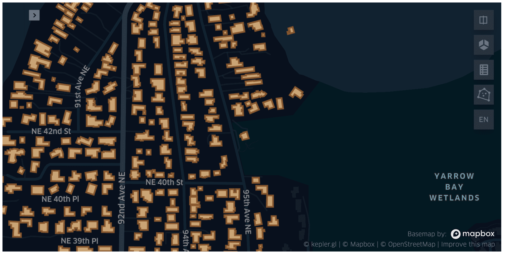
Then we'll define a spatial filter for the city of Bellevue in Washington and use this filter to query the Overture dataset for all buildings in the city of Bellevue.
# Bellevue city boundary
spatial_filter = "POLYGON ((-122.235128 47.650163, -122.233796 47.65162, -122.231581 47.653287, -122.228514 47.65482, -122.227526 47.655204, -122.226175 47.655729, ... -122.23322999999999 47.638110999999995, -122.233239 47.638219, -122.233262 47.638279, -122.233313 47.638324999999995, -122.233255 47.638359, -122.233218 47.638380999999995, -122.233153 47.638450999999996, -122.233136 47.638552999999995, -122.233137 47.638692, -122.232715 47.639348999999996, -122.232659 47.640093, -122.232704 47.641375, -122.233821 47.645111, -122.234906 47.648874, -122.234924 47.648938, -122.235128 47.650163))"
df_building = sedona.read.format("geoparquet").load(DATA_LINK+"theme=buildings/type=building")
df_building = df_building.filter("ST_Contains(ST_GeomFromWKT('"+spatial_filter+"'), geometry) = true")
We can visualize this building data using the Kepler.gl integration with Sedona.
map_building = SedonaKepler.create_map(df_building, 'Building')

map_building
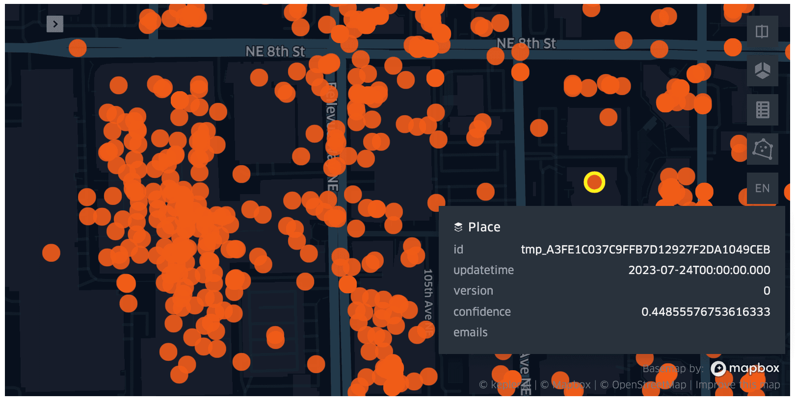
Next, we'll apply the same spatial filter to the "places" Overture theme to find all points of interest within the city of Bellevue. Note the use of the ST_Contains SQL predicate and the ST_GeomFromWKT SQL function.
df_place = sedona.read.format("geoparquet").load(DATA_LINK+"theme=places/type=place")
df_place = df_place.filter("ST_Contains(ST_GeomFromWKT('"+spatial_filter+"'), geometry) = true")
map_place = SedonaKepler.create_map(df_place, "Place")

map_place
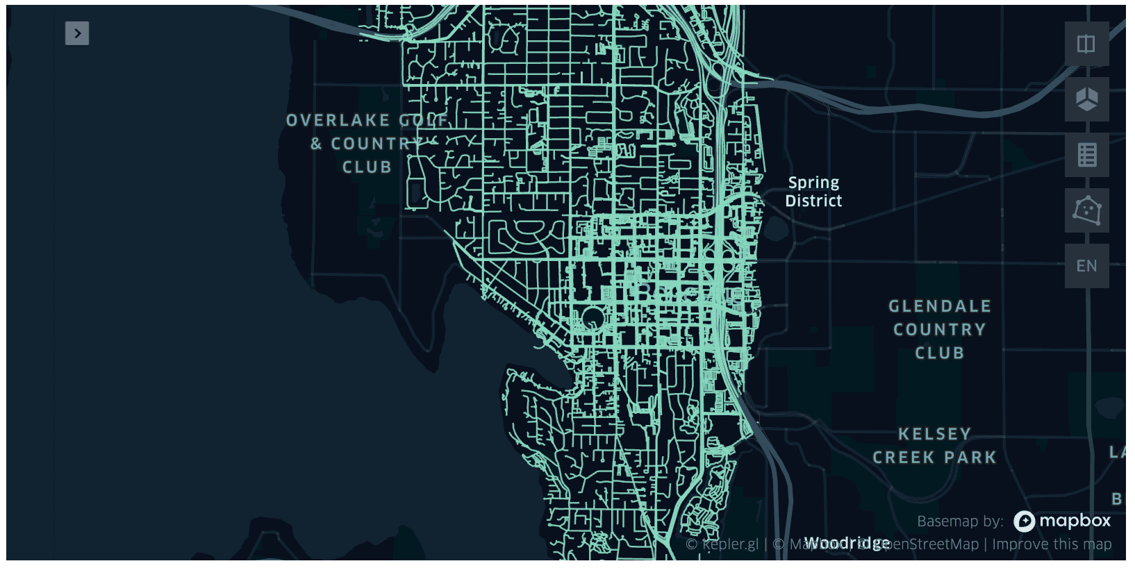
One of the more interesting aspects of the Overture dataset is the "transportation" theme which can be used for use cases like routing and mapping. This theme is split into two pieces: segments and connectors. Connectors represent point geometries where a physical connection between two or more segments occur (think of these as intersections in a routing graph essentially). Segments represent a line geometry and describe the shape of a piece of the transportation network (such as a road or trail).
We can load the segments from the transportation theme, again using the same spatial filter and visualize them using Kepler in our notebook environment.
df_segment = sedona.read.format("geoparquet").load(DATA_LINK+"theme=transportation/type=segment")
df_segment = df_segment.filter("ST_Contains(ST_GeomFromWKT('"+spatial_filter+"'), geometry) = true")
map_segment = SedonaKepler.create_map(df_segment, "Segment")
map_segment
ApacheSedonaRaster.ipynb#
So far we've been working with vector data, but we can also work with raster data in Apache Sedona for use cases such as working with aerial imagery, weather models, and other raster products.
Here we load our raster data stored as geotiff images.
# Path to directory of geotiff images
DATA_DIR = "./data/raster/"
df = sedona.read.format("geotiff").option("dropInvalid",True).option("readToCRS", "EPSG:4326").option("disableErrorInCRS", False).load(DATA_DIR)
df.printSchema()
root
|-- image: struct (nullable = true)
| |-- origin: string (nullable = true)
| |-- geometry: string (nullable = true)
| |-- height: integer (nullable = true)
| |-- width: integer (nullable = true)
| |-- nBands: integer (nullable = true)
| |-- data: array (nullable = true)
| | |-- element: double (containsNull = true)
Much of the functionality for working with raster data in Apache Sedona is available in SedonaSQL as functions prepended with RS_
'''RS_GetBand() will fetch a particular band from given data array which is the concatenation of all the bands'''

df = df.selectExpr("Geom","RS_GetBand(data, 1,bands) as Band1","RS_GetBand(data, 2,bands) as Band2","RS_GetBand(data, 3,bands) as Band3", "RS_GetBand(data, 4,bands) as Band4")
df.createOrReplaceTempView("allbands")
df.show(5)
+--------------------+--------------------+--------------------+--------------------+--------------------+
| Geom               | Band1              | Band2              | Band3              | Band4              |
+--------------------+--------------------+--------------------+--------------------+--------------------+
|POLYGON ((-58.702...|[1081.0, 1068.0, ...|[909.0, 909.0, 82...|[677.0, 660.0, 66...|[654.0, 652.0, 66...|
|POLYGON ((-58.286...|[1151.0, 1141.0, ...|[894.0, 956.0, 10...|[751.0, 802.0, 87...|[0.0, 0.0, 0.0, 0...|
+--------------------+--------------------+--------------------+--------------------+--------------------+
For example, functions like RS_NormalizedDifference which can be used to calculate NDVI, a measure of vegetative health when looking at landcover use cases.
NomalizedDifference = df.selectExpr("RS_NormalizedDifference(Band1, Band2) as normDiff")
NomalizedDifference.show(5)
+--------------------+
| normDiff           |
+--------------------+
|[-0.09, -0.08, -0...|
|[-0.13, -0.09, -0...|
+--------------------+
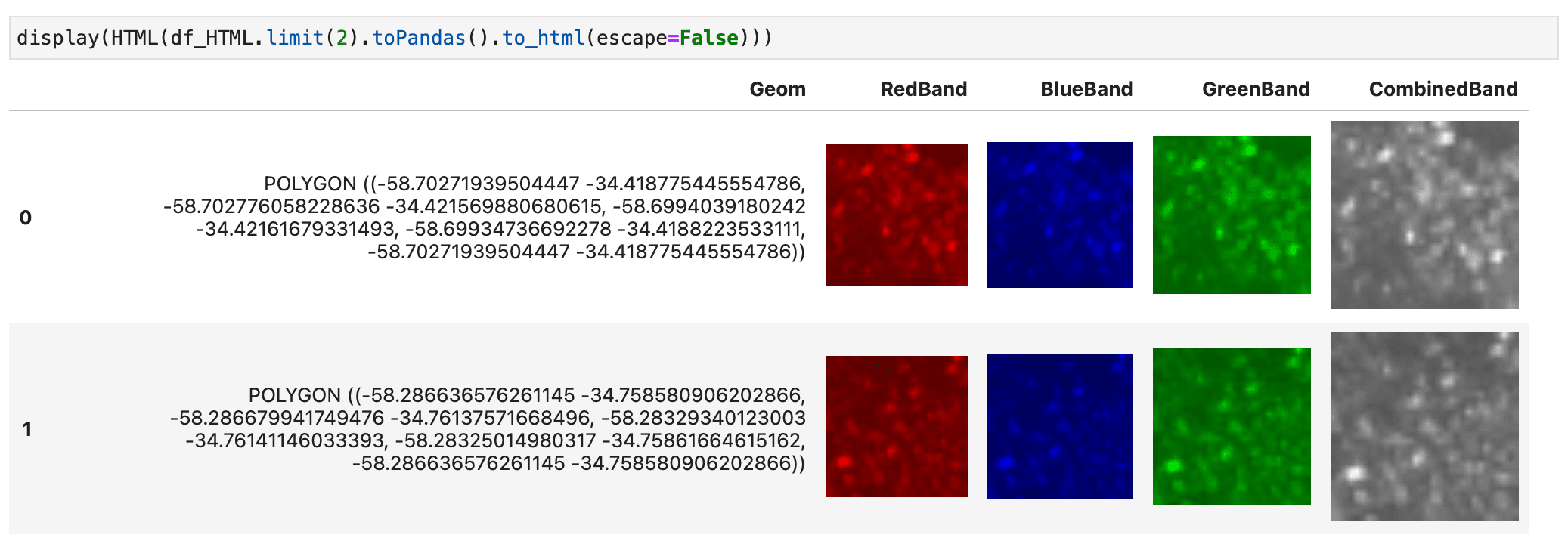
There are a number of other map algebra SQL functions available with Apache Sedona's raster support. Here we select and manipulate various bands of our raster data and visualize them in our notebook environment.
df = sedona.read.format("geotiff").option("dropInvalid",True).option("readToCRS", "EPSG:4326").load(DATA_DIR)
df = df.selectExpr("image.origin as origin","ST_GeomFromWkt(image.geometry) as Geom", "image.height as height", "image.width as width", "image.data as data", "image.nBands as bands")

df = df.selectExpr("RS_GetBand(data,1,bands) as targetband", "height", "width", "bands", "Geom")
df_base64 = df.selectExpr("Geom", "RS_Base64(height,width,RS_Normalize(targetBand), RS_Array(height*width,0.0), RS_Array(height*width, 0.0)) as red","RS_Base64(height,width,RS_Array(height*width, 0.0), RS_Normalize(targetBand), RS_Array(height*width, 0.0)) as green", "RS_Base64(height,width,RS_Array(height*width, 0.0),  RS_Array(height*width, 0.0), RS_Normalize(targetBand)) as blue","RS_Base64(height,width,RS_Normalize(targetBand), RS_Normalize(targetBand),RS_Normalize(targetBand)) as RGB" )
df_HTML = df_base64.selectExpr("Geom","RS_HTML(red) as RedBand","RS_HTML(blue) as BlueBand","RS_HTML(green) as GreenBand", "RS_HTML(RGB) as CombinedBand")
df_HTML.show(5)
Now that we've reviewed the Jupyter notebooks that ship with the Apache Sedona docker image let's create a new notebook, load some of our own data and perform some basic geoprocessing steps. I've been working on a project with some hydrological data so I'll create a new notebook called BasinGeoprocessing.ipynb.
BasinGeoprocessing.ipynb#
First we'll import the sedona.spark.* dependencies and some initial setup to point Sedona at our local Spark cluster.
from sedona.spark import *

config = SedonaContext.builder().master("spark://localhost:7077").getOrCreate()
sedona = SedonaContext.create(config)

sc = sedona.sparkContext
When I started the Docker container I used the -v flag to mount a volume mapping the geodata/ directory in the container to a directory on my local machine where I've stored some Shapefiles of water basin data downloaded from the HydroSHEDs project.
We'll use the ShapefileReader to import one of these shapefiles into a Polygon Spatial RDD, then convert the Spatial RDD to a Spatial DataFrame so we can query it using Spatial SQL. Let's print the schema so we can see what fields we're working with.
hucs = ShapefileReader.readToGeometryRDD(sc, "geodata/basins")
hucs_df = Adapter.toDf(hucs, sedona)
hucs_df.createOrReplaceTempView("basins")
hucs_df.printSchema()
root
|-- geometry: geometry (nullable = true)
|-- HYBAS_ID: string (nullable = true)
|-- NEXT_DOWN: string (nullable = true)
|-- NEXT_SINK: string (nullable = true)
|-- MAIN_BAS: string (nullable = true)
|-- DIST_SINK: string (nullable = true)
|-- DIST_MAIN: string (nullable = true)
|-- SUB_AREA: string (nullable = true)
|-- UP_AREA: string (nullable = true)
|-- PFAF_ID: string (nullable = true)
|-- ENDO: string (nullable = true)
|-- COAST: string (nullable = true)
|-- ORDER: string (nullable = true)
|-- SORT: string (nullable = true)
And let's also look at the first 10 rows to see what the data looks like. Note that we're working with polygon geometries.
hucs_df.show(10)
+--------------------+----------+---------+----------+----------+---------+---------+--------+--------+-------+----+-----+-----+----+
| geometry           | HYBAS_ID |NEXT_DOWN| NEXT_SINK| MAIN_BAS |DIST_SINK|DIST_MAIN|SUB_AREA| UP_AREA|PFAF_ID|ENDO|COAST|ORDER|SORT|
+--------------------+----------+---------+----------+----------+---------+---------+--------+--------+-------+----+-----+-----+----+
|MULTIPOLYGON (((-...|7040000010|        0|7040000010|7040000010|      0.0|      0.0|227171.7|227171.7|   7711|   0|    1|    0|   1|
|POLYGON ((-98.641...|7040005410|        0|7040005410|7040005410|      0.0|      0.0|116984.0|116984.0|   7712|   0|    0|    1|   2|
|MULTIPOLYGON (((-...|7040005420|        0|7040005420|7040005420|      0.0|      0.0| 61109.5| 61109.5|   7713|   0|    1|    0|   3|
|POLYGON ((-102.34...|7040006390|        0|7040006390|7040006390|      0.0|      0.0|134071.8|134071.8|   7714|   0|    0|    1|   4|
|MULTIPOLYGON (((-...|7040006400|        0|7040006400|7040006400|      0.0|      0.0|116166.9|116166.9|   7715|   0|    1|    0|   5|
|POLYGON ((-108.36...|7040007380|        0|7040007380|7040007380|      0.0|      0.0| 34844.5| 34844.5|   7716|   0|    0|    1|   6|
|MULTIPOLYGON (((-...|7040007390|        0|7040007390|7040007390|      0.0|      0.0| 25272.6| 25272.6|   7717|   0|    1|    0|   7|
|POLYGON ((-109.93...|7040007830|        0|7040007830|7040007830|      0.0|      0.0| 77326.4| 77326.4|   7718|   0|    0|    1|   8|
|MULTIPOLYGON (((-...|7040007840|        0|7040007840|7040007840|      0.0|      0.0|116227.8|116227.8|   7719|   0|    1|    0|   9|
|POLYGON ((-114.95...|7040008710|        0|7040008710|7040008710|      0.0|      0.0|  5056.9|620437.5|   7721|   0|    0|    1|  10|
+--------------------+----------+---------+----------+----------+---------+---------+--------+--------+-------+----+-----+-----+----+
only showing top 10 rows
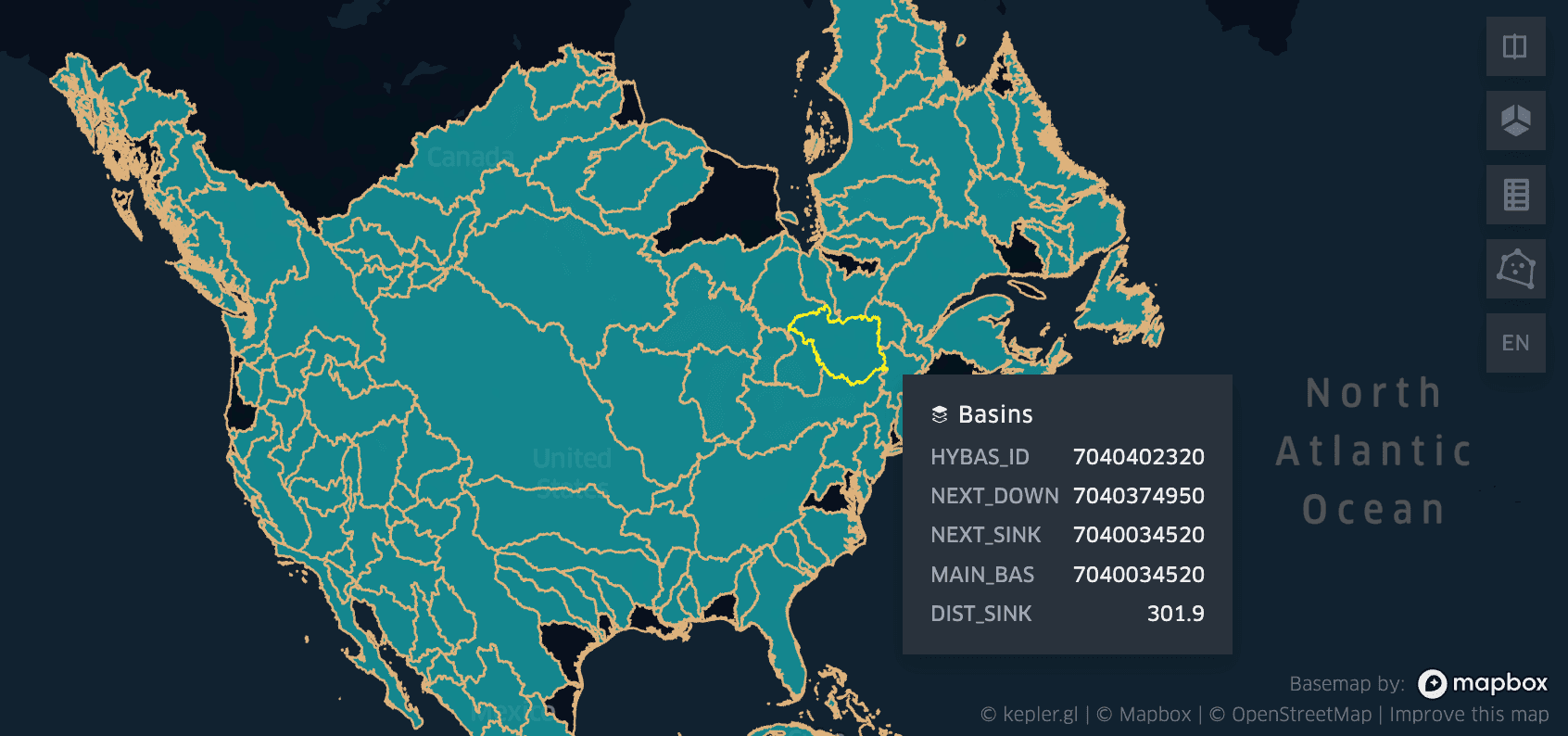
We can also use the SedonaKepler Kepler.gl integration to visualize our spatial data in a map view.
basins_map = SedonaKepler.create_map(hucs_df, "basins")
basins_map
Now that we've loaded our data, let's use SedonaSQL to calculate the centroid for each water basin polygon using the ST_Centroid SQL function.
SELECT ST_Centroid(geometry) AS centroid, * FROM basins
We'll also bring through all the fields for each row.
centroids_df = sedona.sql("SELECT ST_Centroid(geometry) AS centroid, * FROM basins")
centroids_df.show(10)
+--------------------+--------------------+----------+---------+----------+----------+---------+---------+--------+--------+-------+----+-----+-----+----+
| centroid           | geometry           | HYBAS_ID |NEXT_DOWN| NEXT_SINK|  MAIN_BAS|DIST_SINK|DIST_MAIN|SUB_AREA| UP_AREA|PFAF_ID|ENDO|COAST|ORDER|SORT|
+--------------------+--------------------+----------+---------+----------+----------+---------+---------+--------+--------+-------+----+-----+-----+----+
|POINT (-90.708864...|MULTIPOLYGON (((-...|7040000010|        0|7040000010|7040000010|      0.0|      0.0|227171.7|227171.7|   7711|   0|    1|    0|   1|
|POINT (-99.959487...|POLYGON ((-98.641...|7040005410|        0|7040005410|7040005410|      0.0|      0.0|116984.0|116984.0|   7712|   0|    0|    1|   2|
|POINT (-104.10395...|MULTIPOLYGON (((-...|7040005420|        0|7040005420|7040005420|      0.0|      0.0| 61109.5| 61109.5|   7713|   0|    1|    0|   3|
|POINT (-102.47688...|POLYGON ((-102.34...|7040006390|        0|7040006390|7040006390|      0.0|      0.0|134071.8|134071.8|   7714|   0|    0|    1|   4|
|POINT (-106.22590...|MULTIPOLYGON (((-...|7040006400|        0|7040006400|7040006400|      0.0|      0.0|116166.9|116166.9|   7715|   0|    1|    0|   5|
|POINT (-107.82836...|POLYGON ((-108.36...|7040007380|        0|7040007380|7040007380|      0.0|      0.0| 34844.5| 34844.5|   7716|   0|    0|    1|   6|
|POINT (-109.22625...|MULTIPOLYGON (((-...|7040007390|        0|7040007390|7040007390|      0.0|      0.0| 25272.6| 25272.6|   7717|   0|    1|    0|   7|
|POINT (-109.10711...|POLYGON ((-109.93...|7040007830|        0|7040007830|7040007830|      0.0|      0.0| 77326.4| 77326.4|   7718|   0|    0|    1|   8|
|POINT (-111.79932...|MULTIPOLYGON (((-...|7040007840|        0|7040007840|7040007840|      0.0|      0.0|116227.8|116227.8|   7719|   0|    1|    0|   9|
|POINT (-114.91109...|POLYGON ((-114.95...|7040008710|        0|7040008710|7040008710|      0.0|      0.0|  5056.9|620437.5|   7721|   0|    0|    1|  10|
+--------------------+--------------------+----------+---------+----------+----------+---------+---------+--------+--------+-------+----+-----+-----+----+
only showing top 10 rows
Now that we've calculated the centroid for each basin we're ready to export our data to GeoJSON so we can import the data into the other system we're working with that supports point geometries.
centroid_rdd = Adapter.toSpatialRdd(centroids_df, "centroid")
centroid_rdd.saveAsGeoJSON("geodata/huc_centroids2")
That was a quick look at getting started with Apache Sedona via the Apache Sedona Docker image. We've only just scratched the surface here of what we can do with Sedona. I'll be sharing more as I continue my journey. Please reach out if you have ideas for how we can help you work with spatial data to solve your spatial problems!
Resources#
Stay Updated
Get notified about new posts and videos
